R CSV Files
R CSV Files
Leave a reply

R CSV Files
The inheritance is one of the important feature in object oriented programming, that facilitates the code re-usability. Inheritance is a mechanism through which a class(derived class) can inherit properties and methods from an existing class(base class).
Sub Class:- The class that inherits properties and methods from another class is know as Sub-class or Derived-Class.
Super Class:- The class whose properties and methods are being inherited by sub class is called Base Class or Super class.
Reference class is basically a S4 class with an environment added to it.
In R, reference classes are defined using the setRefClass() function.
Syntax:-
|
1 |
setRefClass("ReffClassName") |
Example:-
|
1 |
setRefClass("employee") |
Class can be defined as a blueprint or prototype of associated objects. Class wrapper that binds the data and methods which can be later accessed by objects of that class. We can think of a class as a user-defined data type, that describes the behavior and characteristics shared by all of its instances. Once a class has been defined, we can create instance or objects of that class which has access to class properties and methods.
In R, before we perform any analysis over data provided, it must be changed it into required format. Data Reshaping is the process about changing the way data is organized into rows and columns. In data reshaping we take input data as data frame and change or reshape it into required format. Sometimes we may need to convert input data into intermediate format in order to reshape it in required data format.
R comes with a rich set of functions for reshaping data prior to analysis including functions to split, merge and change the rows to columns and vice-versa in a data frame.
The t() function is used to transpose a matrix or a data frame.
Example:-
|
1 2 3 4 5 |
A <- matrix(c(1:9), nrow = 3, byrow = TRUE) A print("W3Adda - After Transpose") A <- t(A) A |
Output:-
In R, we have a “reshape” package which includes a rich set of data reshaping function that makes it easy to perform data analysis.
Reshaping of data may involve multiple steps in order to convert input data into required format. We generally melt data so that each row is converted into unique id-variable combination. Then we cast this data into desired format. The functions used to do this are melt() and cast().
Example:-
Lets take a sample data set as following –
| id | point | x1 | x2 |
| 1 | 1 | 5 | 6 |
| 1 | 2 | 3 | 5 |
| 2 | 1 | 6 | 1 |
| 2 | 2 | 2 | 4 |
Now, lets melt the above data set using melt() function, melt() function will convert all columns other than id and point into multiple rows.
|
1 2 3 |
# example of melt function library(reshape) mdata <- melt(mydata, id=c("id","point")) |
Output:-
| id | point | variable | value |
| 1 | 1 | x1 | 5 |
| 1 | 2 | x1 | 3 |
| 2 | 1 | x1 | 6 |
| 2 | 2 | x1 | 2 |
| 1 | 1 | x2 | 6 |
| 1 | 2 | x2 | 5 |
| 2 | 1 | x2 | 1 |
| 2 | 2 | x2 | 4 |
Now, lets cast the melted data to evaluate mean –
|
1 2 3 4 |
# cast the melted data # cast(data, formula, function) idmeans <- cast(mdata, id~variable, mean) pointmeans <- cast(mdata, point~variable, mean) |
Output:-
idmeans
| id | x1 | x2 |
| 1 | 4 | 5.5 |
| 2 | 4 | 2.5 |
pointmeans
| point | x1 | x2 |
| 1 | 5.5 | 3.5 |
| 2 | 2.5 | 4.5 |
In R, merge() function can be used to merge two data frames. In order to merge data frames they must have same column names on which merging is performed. The merge function is mostly used to merge data frames horizontally. Mostly, merging is performed on one or more common key variables (i.e., an inner join).
Example:-
|
1 2 3 4 |
# merge two data frames by ID total <- merge(dfA,dfB,by="ID") # merge two data frames by ID and Country total <- merge(dfA,dfB,by=c("ID","Country")) |
In R, cbind() function is used to join multiple vectors into data frame.
Syntax:-
|
1 |
cbind(x1, x2, ...) |
dfA
| Type | Sex | Exp |
| B | M | 50 |
| A | F | 15 |
dfB
| Age | City |
| 30 | NY |
| 20 | SF |
Example:-
|
1 |
dfC <- cbind(dfA,dfB) |
Output:-
| Type | Sex | Exp | Age | City |
| B | M | 50 | 30 | NY |
| A | F | 15 | 20 | SF |
In R, rbind() function is can be used to join multiple data frame.
dfA
| Type | Sex | Exp |
| B | M | 50 |
| A | F | 15 |
dfB
| Type | Sex | Exp |
| D | F | 10 |
| C | M | 5 |
Example:-
|
1 |
dfC <- rbind(dfA,dfB) |
Output:-
| Type | Sex | Exp |
| B | M | 50 |
| A | F | 15 |
| D | F | 10 |
| C | M | 5 |
Package is simply a set of R functions organized in an independent, reusable unit. It usually contains set of functions for a specific purpose or utility along with the complied code and sample data. All of the R packages are stored in library directory. Every R package has its own context, thus it does not interfere with other modules.
R comes with a rich set of default packages, loaded automatically when R console is started. However, any other package other than the default need to be installed and loaded explicitly first in order to use it. Once a packages is loaded, it can be used throughout the R environment.
The .libPaths() function is used to show package directory path.
Example:-
|
1 |
.libPaths() |
Output:-
![]()
The library() function is used to display list of all of the installed package.
Syntax:-
|
1 |
library() |
Output:-
|
1 2 3 4 5 6 7 8 9 10 11 12 13 14 15 16 17 18 19 20 21 22 23 24 25 26 27 28 29 30 31 32 33 34 35 36 37 38 39 40 41 |
Packages in library ‘C:/Program Files/R/R-3.5.1/library’: base The R Base Package boot Bootstrap Functions (Originally by Angelo Canty for S) class Functions for Classification cluster "Finding Groups in Data": Cluster Analysis Extended Rousseeuw et al. codetools Code Analysis Tools for R compiler The R Compiler Package datasets The R Datasets Package foreign Read Data Stored by 'Minitab', 'S', 'SAS', 'SPSS', 'Stata', 'Systat', 'Weka', 'dBase', ... graphics The R Graphics Package grDevices The R Graphics Devices and Support for Colours and Fonts grid The Grid Graphics Package KernSmooth Functions for Kernel Smoothing Supporting Wand & Jones (1995) lattice Trellis Graphics for R MASS Support Functions and Datasets for Venables and Ripley's MASS Matrix Sparse and Dense Matrix Classes and Methods methods Formal Methods and Classes mgcv Mixed GAM Computation Vehicle with Automatic Smoothness Estimation nlme Linear and Nonlinear Mixed Effects Models nnet Feed-Forward Neural Networks and Multinomial Log-Linear Models parallel Support for Parallel computation in R rpart Recursive Partitioning and Regression Trees spatial Functions for Kriging and Point Pattern Analysis splines Regression Spline Functions and Classes stats The R Stats Package stats4 Statistical Functions using S4 Classes survival Survival Analysis tcltk Tcl/Tk Interface tools Tools for Package Development translations The R Translations Package utils The R Utils Package |
The search() function is used to display list of all of the packages currently loaded in the R environment.
Syntax:-
|
1 |
search() |
Output:-
|
1 2 3 |
[1] ".GlobalEnv" "package:stats" "package:graphics" [4] "package:grDevices" "package:utils" "package:datasets" [7] "package:methods" "Autoloads" "package:base" |
In R, there are two ways we can install a new package.
Install using CRAN:-
CRAN is a distributed network around the world that store identical, up-to-date versions of a package code and documentation, which allows you to install a packages from nearest CRAN mirror.Use the following commands to install a R package directly from CRAN mirror –
|
1 2 3 |
install. packages("Package Name") # Install the package named "XML". install. packages ("XML") |
Install Manually:-
Step 1:- Download the R Package directly from the following link –
|
1 |
https://cran.r-project.org/web/packages/available_packages_by_name.html |
Step 2:- Save package zip file in your local system.
Step 3:- Install the package using following commands
|
1 2 3 |
install.packages(file_name_with_path, repos = NULL, type = "source") # Install the package named "XML" install.packages("local_path_to_package_zip_file", repos = NULL, type = "source") |
In R, all of the default packages are loaded automatically when R console is started. However, any other package other than the default need to be installed and loaded explicitly first in order to use it. Once a packages is loaded, it can be used throughout the R environment. In R, a package can be loaded using following commands –
|
1 2 3 |
library("package_name", lib.loc = "path_to_library") # Load the package named "XML" install.packages("local_path_to_package_zip_file", repos = NULL, type = "source") |
Once a package is installed, you may frequently require to update them in order to have an latest package code. A package can be updated using update.packages command as following –
|
1 2 |
update.packages(ask = FALSE) # this won't ask for package updating |
Sometime you may require to delete any package, this can be done using the remove.packages() function as following –
|
1 |
remove.packages("package_name") |
Data Frame is a data structure that contain list of vectors that is of equal length. Vectors in a data frame can be different data types i.e. numeric, character, factor, etc. It is a two dimensional data structure that us mainly used to store data tables.
Example:-
|
1 2 3 4 5 6 |
print("W3Adda - R Data Frame") a <- c(2, 4, 6) b <- c("aaa", "bbb", "ccc") c <- c(TRUE, FALSE, TRUE) df <- data.frame(a, b, c) # df is a data frame print(df) |
Here, df is a data frame containing three vectors a, b, c. When we run the above R script, we see the following output –
Output:-

In Data Frame, each of the component form column and its contents form the rows.
In R, a data frame is created using data.frame() function. The data.frame() function takes a vector input in order to create a factor.
Syntax:-
|
1 |
data.frame(df, stringsAsFactors = TRUE) |
Above is the general syntax of data.frame() function, here
df:- It is collection of vector input that us being join as data frame, or it could be a matrix that can be converted to data frame.
stringsAsFactors:- It convert string to factor by default. To suppress this behavior, we can pass assign FALSE to it.
Let’s create a data frame using data.frame() function –
Example:-
|
1 2 3 4 5 6 |
print("W3Adda - R Data Frame") a <- c(2, 4, 6) b <- c("aaa", "bbb", "ccc") c <- c(TRUE, FALSE, TRUE) df <- data.frame(a, b, c) # df is a data frame print(df) |
Here, df is a data frame containing three vectors a, b, c. When we run the above R script, we see the following output –
Output:-
Elements in a data frame can be accessed same way as of list or matrix by passing row and column index value(s) in brackets [ ] separated with a comma you can access individual data frame element. However, individual column can be accessed using [[ or $ operator.
Syntax:-
|
1 |
df[row,col] |
df:- Data frame name
row:- row index of the element, if not provided specified row elements will be fetched for all columns.
col:- column index of the element, if not provided specified column elements will be fetched for all rows.
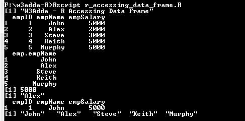
Example:-
|
1 2 3 4 5 6 7 8 9 10 11 12 13 14 15 16 17 18 19 20 21 22 23 24 |
print("W3Adda - R Accessing Data Frame") # Create the data frame. emp <- data.frame( empID = c (1:5), empName = c("John","Alex","Steve","Keith","Murphy"), empSalary = c(5000,2000,3000,5000,5000), stringsAsFactors = FALSE ) print(emp) # Access Specific columns. A <- data.frame(emp$empName) print(A) # Access the element at 1st row and 3rd column. print(emp[1,3]) # Access the element at 2nd row and 5th column. print(emp[2,2]) # Access only the 1st row. print(emp[1,]) # Access only the 5th column. print(emp[,2]) |
When we run the above R script, we see the following output –
Output:-
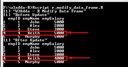
A data frame element can be modified by accessing element using above method and assigning it new value.
Example:-
|
1 2 3 4 5 6 7 8 9 10 11 12 13 |
print("W3Adda - R Modify Data Frame") # Create the data frame. emp <- data.frame( empID = c (1:5), empName = c("John","Alex","Steve","Keith","Murphy"), empSalary = c(5000,2000,3000,5000,5000), stringsAsFactors = FALSE ) print("Before Update") print(emp) print("After Update") emp[4,3] <- 4000 print(emp) |
Output:-
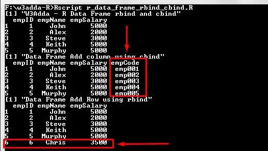
The rbind() and cbind()function is used to add a row and column respectively to a data frame.
Example:-
|
1 2 3 4 5 6 7 8 9 10 11 12 13 |
print("W3Adda - R Data Frame rbind and cbind") # Create the data frame. emp <- data.frame( empID = c (1:5), empName = c("John","Alex","Steve","Keith","Murphy"), empSalary = c(5000,2000,3000,5000,5000), stringsAsFactors = FALSE ) print(emp) print("Data Frame Add column using cbind") cbind(emp, "empCode" = c("emp001", "emp002", "emp003", "emp004", "emp005")) # add column print("Data Frame Add Row using rbind") rbind(emp, c(6, "Chris", 3500)) # add row |
Output:-
A data frame element can be deleted by simply accessing and assigning NULL value to it.
Factor is a data structure that can only contain predefined set of values(categorical data). Factors are useful when we want deal with limited set of values for variable, in this case we must define the possible values beforehand and all of the distinct values are termed as levels.
Example:-
|
1 2 3 |
print("W3Adda - R Factors") dow <- factor(c("Sunday", "Monday", "Tuesday", "Wednesday", "Thursday", "Friday", "Saturday")) dow |
Here, we have defined a factor that contains all of 7 weekdays as values.
Output:-
When we run the above R script, we see the following output –
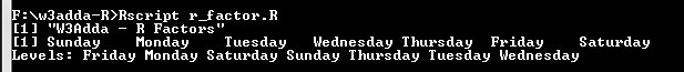
It list all of the factor values and levels. It has the 7 levels.
In R, a factor is created using factor() function. The factor() function takes a vector input in order to create a factor.
Syntax:-
|
1 |
factor(data, levels = lData) |
Above is the general syntax of factor() function, here
data:- It is a vector input which contains all of the factor values.
levels:- It takes a vector input(lData) which contains all of the factor levels. Levels can be inferred from the data if not provided.
Example:-
|
1 2 3 |
print("W3Adda - R Creating Factor") s <- factor(c("Red", "Green", "Yellow", "Red"), levels = c("Red", "Green", "Yellow")) s |
Output:-

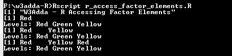
Factor elements can be accessed same way as of vectors, by passing index value(s) in brackets [ ] you can access factor elements. An index value can be logical, integer or character.
Example:-
|
1 2 3 4 5 6 7 8 9 10 |
print("W3Adda - R Accessing Factor Elements") t <- factor(c("Red", "Green", "Yellow", "Red"), levels = c("Red", "Green", "Yellow")) # Accessing 1st factor elements using integer indexing. t[c(1)] # Accessing 1st and 3rd factor elements using integer indexing. t[c(1,3)] # Accessing 1st, 3rd and 4th factor elements using logical indexing. t[c(TRUE, FALSE, TRUE, TRUE)] |
Output:-
A factor element can be modified by accessing element and assigning it new value from predefined set of values.
Example:-
|
1 2 3 4 5 6 7 |
print("W3Adda - R Update Factor Element") t <- factor(c("Red", "Green", "Yellow", "Red"), levels = c("Red", "Green", "Yellow")) print("Factor Element Before Update") print(t[4]) print("Factor Element After Update") t[4] <- "Green" print(t[4]) |
Output:-
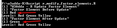
Note:- If we try to assign values outside of its predefined levels, then it raise an error.
Array is a data structure that enable you to store multi dimensional(more than 2 dimensions) data of same type. In R, an array of (2, 3, 2) dimension contains 2 matrix of 2×3.
In R, an array can be created using the array() function as following –
Syntax:-
|
1 |
array(data, dim) |
Above is the general syntax of array() function, here
data:- It is a vector input used to create array.
dim:- It is used to represent array dimensions.
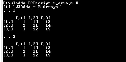
Example:-
|
1 2 3 4 5 6 7 |
print("W3Adda - R Arrays") # Two vectors of different lengths. a <- c(1,2,3) b <- c(10,11,12,13,14,15) # Take vectors as input and creats array. arr <- array(c(a,b),dim = c(3,3,2)) print(arr) |
Output:-
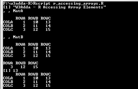
The dimnames parameter in array() function is used to give names to the rows, columns along with matrices.
Example:-
|
1 2 3 4 5 6 7 8 9 |
print("W3Adda - R Naming Arrays") # Two vectors of different lengths. a <- c(1,2,3) b <- c(10,11,12,13,14,15) column.names <- c ("COLA","COLB","COLC") row.names <- c ("ROWA","ROWB","ROWC") matrix.names <- c ("MatA", "MatB") arr <- array (c (a,b), dim=c (3,3,2), dimnames=list (column.names, row.names, matrix.names)) print(arr) |
Output:-

Array elements can be accessed by using the row and column index of the element as following –
Syntax:-
|
1 |
arr[row,col,matrix] |
arr:- Array name
row:- row index of the element, if not provided specified row elements will be fetched for all columns.
col:- column index of the element, if not provided specified column elements will be fetched for all rows.
matrix:- matrix index.
Example:-
|
1 2 3 4 5 6 7 8 9 10 11 12 13 14 15 16 17 18 19 |
print("W3Adda - R Accessing Array Elements") # Two vectors of different lengths. a <- c(1,2,3) b <- c(10,11,12,13,14,15) column.names <- c ("COLA","COLB","COLC") row.names <- c ("ROWA","ROWB","ROWC") matrix.names <- c ("MatA", "MatB") arr <- array (c (a,b), dim=c (3,3,2), dimnames=list (column.names, row.names, matrix.names)) print(arr) # Print the third row of the second matrix of the array. print(arr[3,,2]) # Print the element in the 1st row and 3rd column of the 1st matrix. print(arr[1,3,1]) # Print the 2nd Matrix. print(arr[,,2]) |
When we run the above R script, we see the following output –
Output:-
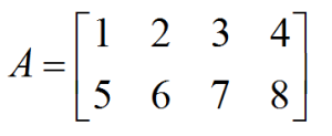
Matrix is a two dimensional data structure, where elements are arranged in rows and columns. It can thought as combination of two or more vectors of same data type. Following is an example of a 2×4 matrix with 2 rows and 4 columns.
A matrix is created using the matrix() function. The values for matrix rows and matrix columns is defined using nrow and ncol arguments. However, it is not required to provide value for both as it automatically evaluate the value for other dimension using length of matrix.
Syntax:-
|
1 |
matrix(data, nrow, ncol, byrow = FALSE) |
Above is the general syntax of matrix() function, here
data:- It is a vector input which will arranged as matrix.
nrow:- Number of rows.
ncol:- Number of columns.
byrow:- If it is TRUE values being filled by row (left to right). If it is FALSE values being filled by Column(top to bottom). Default is FALSE.
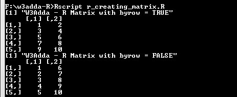
Example:-
Here we are creating two 5×2 matrix which contains number from 1 to 10 keeping byrow = TRUE for and byrow = FALSE for other to check the difference.
|
1 2 3 4 5 6 |
print("W3Adda - R Matrix with byrow = TRUE") matrixA <- matrix(c(1:10), nrow = 5, byrow = TRUE) matrixA print("W3Adda - R Matrix with byrow = FALSE") matrixB <- matrix(c(1:10), nrow = 5, byrow = FALSE) matrixB |
Output:-
Matrix elements can be accessed by using the row and column index of the element as following –
Syntax:-
|
1 |
matrix[row,col] |
matrix:- Matrix name
row:- row index of the element, if not provided specified row elements will be fetched for all columns.
col:- column index of the element, if not provided specified column elements will be fetched for all rows.
Example:-
Let’s have a 3×5 matrix which contains number from 1 to 15 keeping byrow = TRUE. Now, we are accessing different matrix elements as following –
|
1 2 3 4 5 6 7 8 9 10 11 12 13 14 |
print("W3Adda - R Access Matrix Elements") A <- matrix(c(1:15), nrow = 3, byrow = TRUE) A # Access the element at 1st row and 3rd column. print(A[1,3]) # Access the element at 2nd row and 5th column. print(A[2,5]) # Access only the 1st row. print(A[1,]) # Access only the 5th column. print(A[,5]) |
When we run the above R script, we see the following output –
Output:-

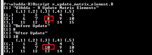
A matrix element can be modified by accessing element using above method and assigning it new value.
Example:-
|
1 2 3 4 5 6 7 8 9 |
print("W3Adda - R Update Matrix Elements") A <- matrix(c(1:15), nrow = 3, byrow = TRUE) A print("Before Update") print(A[2,3]) print("After Update") A[2,3] <- 10 print(A[2,3]) A |
Output:-
The rbind() and cbind()function is used to add a row and column respectively to a matrix.
Example:-
|
1 2 3 4 5 6 |
A <- matrix(c(1:9), nrow = 3, byrow = TRUE) A print("W3Adda - Matrix Add One Column") cbind(A, c(1, 2, 3)) # add column print("W3Adda - Matrix Add One Row") rbind(A,c(1,2,3)) # add row |
Output:-

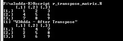
The t() function is used to transpose a matrix.
Example:-
|
1 2 3 4 5 |
A <- matrix(c(1:9), nrow = 3, byrow = TRUE) A print("W3Adda - After Transpose") A <- t(A) A |
Output:-
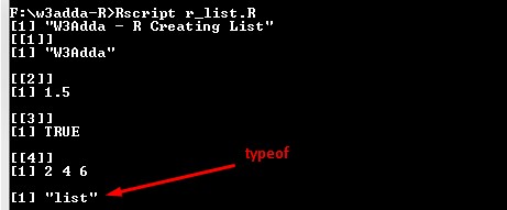
List is a basic data structure that can contain elements of different types. It is similar to vectors except it can contains mixed data i.e. numbers, strings, vectors and another list inside it.
Example:-
|
1 |
list(1.5, TRUE, c(2,4,6)) |
A list can be created using list() function as following –
Example:-
Following is an example to create a list containing strings, numbers, vectors and a logical values.
|
1 2 3 4 |
print("W3Adda - R Creating List") x <- list("W3Adda", 1.5, TRUE, c(2,4,6)) print(x) typeof(x) |
Output:-
In R, we can assign name or tags to the list elements, that makes it easy to reference the individual element of the list.
Example:-
Following is an example to create same list with the tags as follows.
|
1 |
x <- list("a" = 1.5, "b" = TRUE, "c" = c(2,4,6)) |
Here,
a, b and c are tags which makes it easier to reference the respective list element.
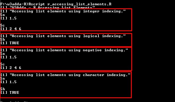
List elements can be accessed in same as of vectors. An index value can be logical, integer or character.
Example:-
|
1 2 3 4 5 6 7 8 9 10 11 12 13 14 15 16 17 18 19 20 21 22 |
print("W3Adda - R Accessing List Elements") # Accessing list elements using integer indexing. t <- list("a" = 1.5, "b" = TRUE, "c" = c(2,4,6)) u <- t[c(1,3)] print("Accessing list elements using integer indexing.") print(u) # Accessing list elements using logical indexing. v <- t[c(FALSE,TRUE,FALSE)] print("Accessing list elements using logical indexing.") print(v) # Accessing list elements using negative indexing. x <- t[c(-2)] print("Accessing list elements using negative indexing.") print(x) # Accessing list elements using character indexing. b <- t[c("a","b")] print("Accessing list elements using character indexing.") print(b) |
Output:-
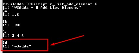
An element can be simply added by assigning a values with new tags.
Example:-
|
1 2 3 4 |
print("W3Adda - R Add List Element") x <- list("a" = 1.5, "b" = TRUE, "c" = c(2,4,6)) x['d'] <- "w3adda" print(x) |
Here, we have added a new list element with “d” tag and assigning it value “w3adda”. When we run the above R script, we will see following output –
Output:-
A list element can be modified by accessing element and assigning it new value.
Example:-
|
1 2 3 4 5 6 7 |
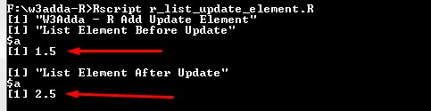
print("W3Adda - R Add Update Element") x <- list("a" = 1.5, "b" = TRUE, "c" = c(2,4,6)) print("List Element Before Update") print(x[1]) print("List Element After Update") x[1] <- 2.5 print(x[1]) |
Here, we have updated list element with index position 1 with new value. When we run the above R script, we will see following output –
Output:-
An element can be simply deleted by assigning NULL value to it.
Example:-
|
1 2 3 4 5 6 7 |
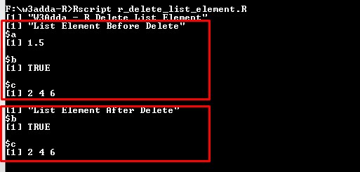
print("W3Adda - R Delete List Element") x <- list("a" = 1.5, "b" = TRUE, "c" = c(2,4,6)) print("List Element Before Delete") print(x) print("List Element After Delete") x[1] <- NULL print(x) |
Here, we have deleted list element with index position 1 by assigning it NULL. When we run the above R script, we will see following output –
Output:-
In R, we can create a new list by merging multiple list using list() function as following –
Example:-
|
1 2 3 4 5 6 7 |
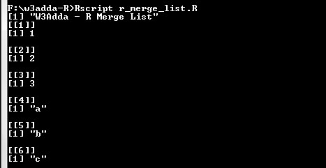
print("W3Adda - R Merge List") list1 <- list(1,2,3) list2 <- list("a","b","c") # Merge the two lists. list3 <- c(list1,list2) # Print the merged list. print(list3) |
Here, we have two list list1 and list2, and we have merge both of the list into list3. When we run the above R script, we will see following output –
Output:-
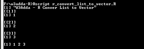
The unlist() function can be used to convert a list object into a vector.
Example:-
|
1 2 3 4 5 |
print("W3Adda - R Conver List to Vector") list1 <- list(1,2,3) print(list1) list2 <- unlist(list1) print(list2) |
Output:-
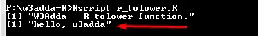
The tolower() function is used to convert given string characters to lower case.
Syntax:-
|
1 |
tolower(str) |
Above is the general syntax of tolower() function, here
str:- It is a vector input representing a string.
Example:-
|
1 2 3 |
print("W3Adda - R tolower function.") result <- tolower("Hello, W3Adda") print(result) |
Output:-